Obtaining summary shap plot for catboost model with tidymodels in R

Question

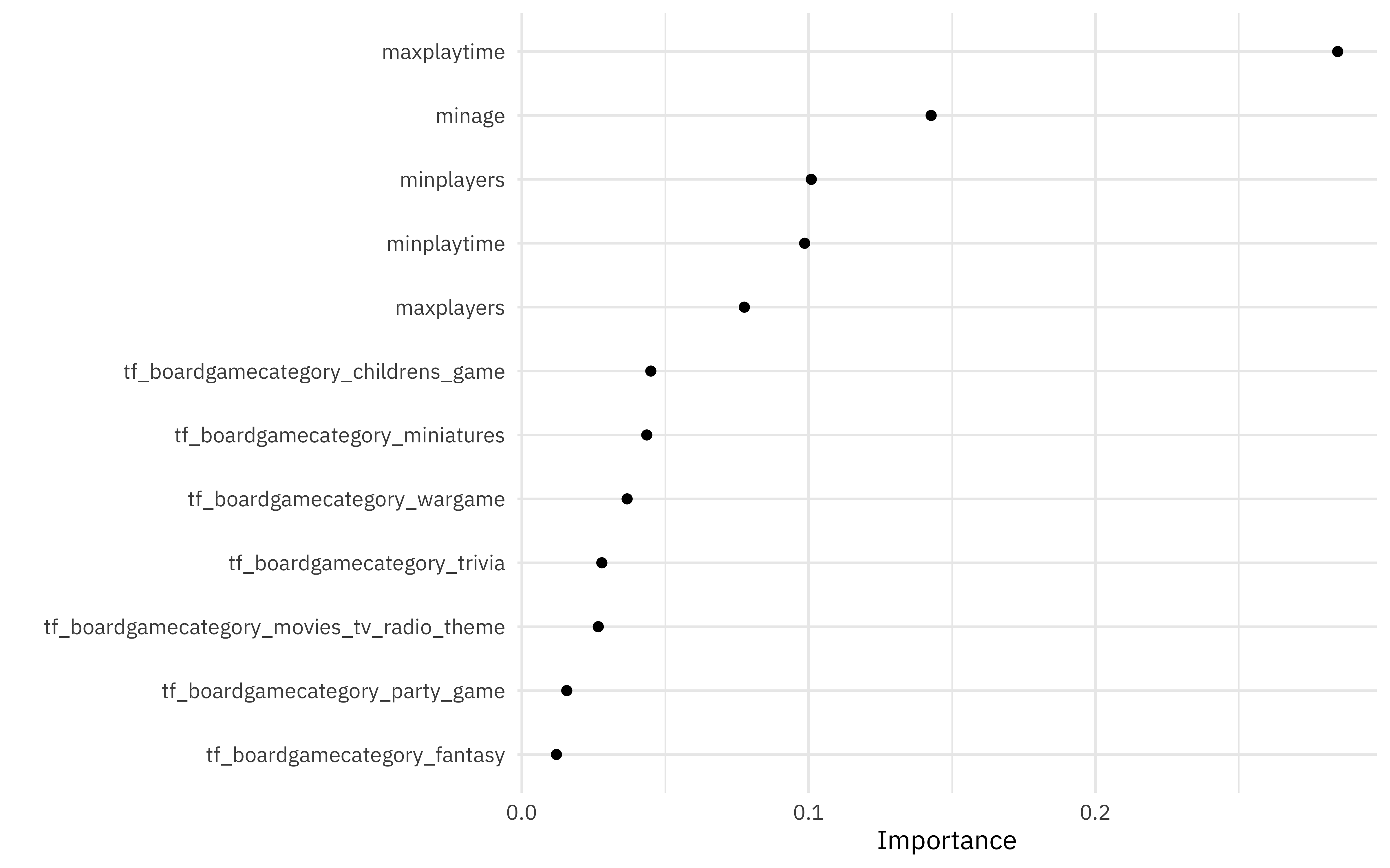
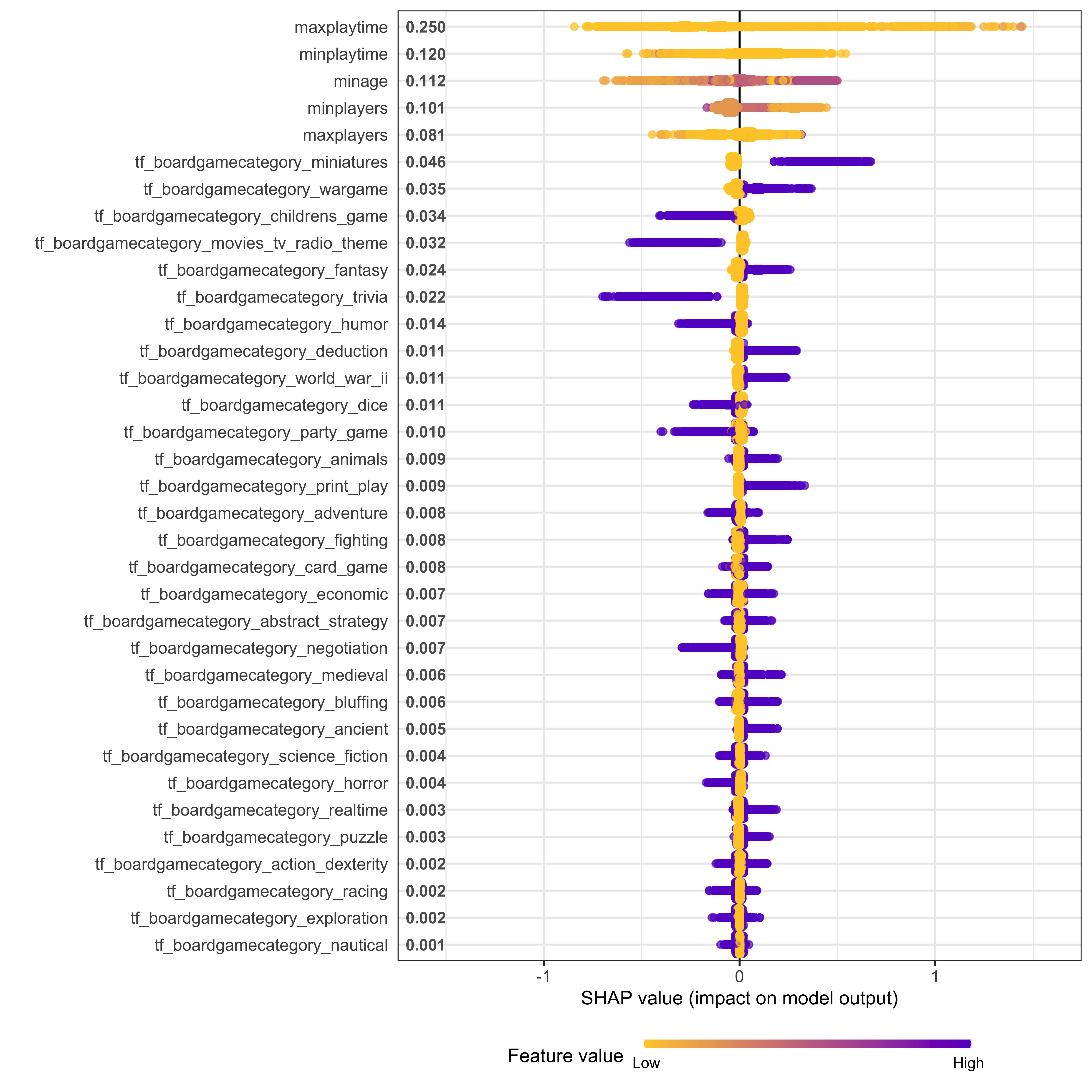
I am trying to build a catboost model within the tidymodels framework. Minimal reproducible example is given below. I am able to use the DALEX and modelStudio packages to get model explanations but I want to create VIP plots like this and summary shap plots like this for this catboost model. I have tried packages like fastshap, SHAPforxgboost without any luck. I realise that i have to extract the variable importance and shap values from the model object and use them to produce these plots but dont know how to do that. Is there a way to get this done in R?

library(tidymodels)
library(treesnip)
library(catboost)
library(modelStudio)
library(DALEXtra)
library(DALEX)

data <- structure(list(Age = c(74, 60, 57, 53, 72, 72, 71, 77, 50, 66), StatusofNation0developed = structure(c(2L, 2L, 2L, 2L, 2L, 
                                                                                                       1L, 2L, 1L, 1L, 2L), .Label = c("0", "1"), class = "factor"), 
               treatment = structure(c(2L, 1L, 2L, 2L, 2L, 1L, 1L, 3L, 1L, 
                                       2L), .Label = c("0", "1", "2"), class = "factor"), InHospitalMortalityMortality = c(0, 
                                                                                                                           0, 1, 1, 1, 0, 0, 1, 1, 0)), row.names = c(NA, 10L), class = "data.frame")
split <- initial_split(data, strata = InHospitalMortalityMortality)
train <- training(split)
test <- testing(split)

train$InHospitalMortalityMortality <- as.factor(train$InHospitalMortalityMortality)

rec <- recipe(InHospitalMortalityMortality ~ ., data = train)

clf <- boost_tree() %>%
  set_engine("catboost") %>%
  set_mode("classification")

wflow <- workflow() %>%
  add_recipe(rec) %>%
  add_model(clf)

model <- wflow %>% fit(data = train)

explainer <- explain_tidymodels(model,
                                data = test,
                                y = test$InHospitalMortalityMortality,
                                label = "catboost")
new_observation <- test[1:2,]
modelStudio(explainer, new_observation)

Answer 1

The link above provides an answer, but it is incomplete. Here it is completed, following an identical workflow.

As indicated: first, install R packages {fastshap} and and {reticulate}. Next, setup a virtual environment for python use with {reticulate}. Setting up a virtual environment is relatively straightforward when using RStudio. Please check their reference material for step by step instructions.

Then, pip install {shap} and {matplotlib} in venv -- note that matplotlib 3.2.2 would seem necessary for summary plots (see GitHub issues for greater detail).

The workflow (from treesnip docs):

library(tidymodels)
library(treesnip)

data("diamonds", package = "ggplot2")
diamonds <- diamonds %>% sample_n(1000)

#vfolds resamples 
diamond_splits <- vfold_cv(diamonds, v = 5)

model_spec <- boost_tree(mtry = 5, trees = 500) %>% set_mode("regression")

#model specifications
lightgbm_model <- model_spec %>% 
    set_engine("lightgbm", nthread = 4)

#workflow
lightgbm_workflow <- workflow() %>% 
    add_model(lightgbm_model)

rec_ordered <- recipe( 
    price ~ .
    ,data = diamonds
)

lightgbm_fit_ordered <- fit_resamples( 
    add_recipe(
        lightgbm_workflow, rec_ordered
    ), resamples = diamond_splits
)

Fit the workflow:

fit_lightgbm_workflow <- lightgbm_workflow %>%
    add_recipe(rec_ordered) %>%
    fit(data = diamonds)

With a fit workflow, we can now create shap values via {fastshap} and plot with {fastshap} and {reticulate}.

First, the force plots: to do this, we need to create a prediction function for the pred_wrapper argument.

predict_function_gbm <- function(model, newdata){
    predict(model, newdata) %>% pull(., 1) # 
}

Now we want the mean prediction values for the baseline argument.

mean_preds <- mean( 
    predict_function_gbm(
      fit_lightgbm_workflow, diamonds %>% select(-price)
      ) 
)

Here, create the shap values:

fastshap::explain( 
  fit_lightgbm_workflow, 
  X = as.data.frame(diamonds %>% select(-price)), 
  pred_wrapper = predict_function_gbm, 
  nsim= 10
) -> gbm_explained

Now, for the force plot:

fastshap::force_plot( 
  object = gbm_explained[1, ],
  feature_values = as.data.frame(diamonds %>% select(-price))[1, ],
  display = "viewer", # or "html" depending on rendering preference
  baseline = mean_preds
)

# For classification, add: link = "logit"
# For vertical stacking, change: [1, ] to [1:20, ] for example. 
# this may or may not throw error depending on version of shap used.
# see {fastshap} issues.

Now for the summary plot: use {reticulate} to access function directly:

library(reticulate)
shap = import("shap")
np = import("numpy")

shap$summary_plot( 
  data.matrix(gbm_explained), 
  data.matrix(diamonds %>% select(-price))
)

The same would work for dependency plots, for example.

shap$dependence_plot( 
  "rank(1)",
  data.matrix(gbm_explained), 
  data.matrix(diamonds %>% select(-price))
)

Final note: repeated rendering will result in buggy visualizations. Naming a feature directly (i.e., "cut") in dependence_plot threw me an error.

Answer 2

First we need to extract the workflow from the model object and use it to predict on the test set.(optional) The used the catboost.load_pool function we create the pool object

predict(model$.workflow[[1]], test[])
pool = catboost.load_pool(dataset, label = label_values, cat_features = NULL)

After this using the catboost.get_feature_importance function we get the feature importance scores on the model object.

catboost.get_feature_importance(extract_fit_engine(model),
                                pool = NULL,
                                type = 'FeatureImportance',
                                thread_count = -1)

Then we can get the shapvalues using the function type = 'ShapValues' option.

shapvalue <- catboost.get_feature_importance(extract_fit_engine(model),
                                             pool = pool,
                                             type = 'ShapValues',
                                             thread_count = -1)
shapvalue <- data.frame(shapvalue)
shap_long_game <- shap.prep(shap_contrib = shapvalue, X_train = dataset)

Finally plot the shapvalues

shap_summplot <- shap.plot.summary(shap_long_game, scientific = F) 
shap_summplot + 
  scale_y_continuous(labels = comma)